Showcase

Here are a few source models and simulation outputs illustrating some of the basic ximpol capabilities.

Cas A

Input model

Full source model definition in ximpol/config/casa.py.

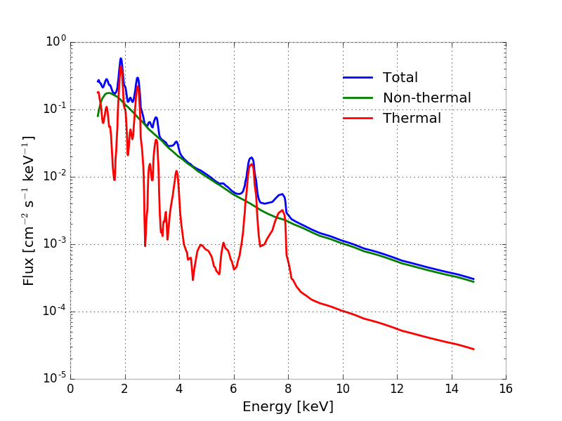
The spectral model is taken (by hand) from Figure 5 of E.A. Helder and J. Vink, “Characterizing the non-thermal emission of Cas A”, Astrophys. J. 686 (2008) 1094–1102. The spectrum of Cas A is a complex superposition of thermal and non thermal emission, and for our purposes, we call thermal anything that is making up for the lines and non-thermal all the rest, as illustrated in the figure below.

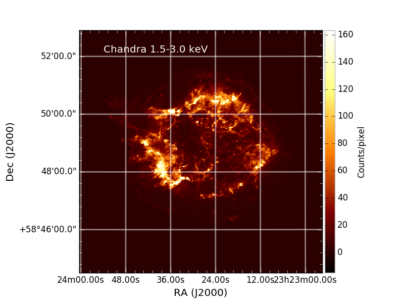
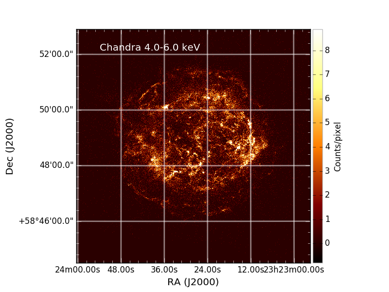
The morphology of the source is energy-dependent in a non trivial way. We start from two Chandra images (in the 1.5–3 keV and 4–6 keV energy ranges, respectively) and associate the former to the thermal spectral component and the latter to the non-thermal one (note the absence of spectral lines between 4 and 6 keV).

For the polarization, we assume that the thermal component is unpolarized, while for the non-thermal component we use a simple geometrical, radially symmetric model (loosely inspired from radio observations) where the polarization angle is tangential and the polarization degree is zero at the center of the source and increases toward the edges reaching about 50% on the outer rim of the source (see figure below).

Our total model of the region of interest is therefore the superposition of two indipendent components, with different spectral, morphological and polarimetric properties. Crude as it is, it’s a good benchmark for the observation simulator.

Simulation output

Generation/analysis pipeline in ximpol/examples/casa.py.

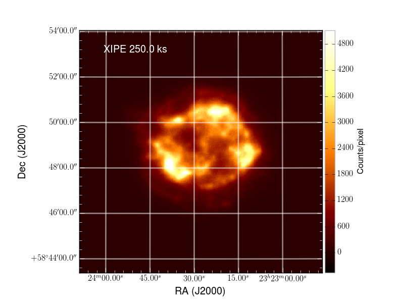
Below is a binned count map of a 250 ks simulated XIPE observation of Cas A, based on the model described above.

When the entire source is analyzed at once, most of the polarization averages out and even in the high-energy band, where the emission is predominantly non-thermal, the residual polarization degree resulting from the averaging of the different emission regions is of the order of 5%.

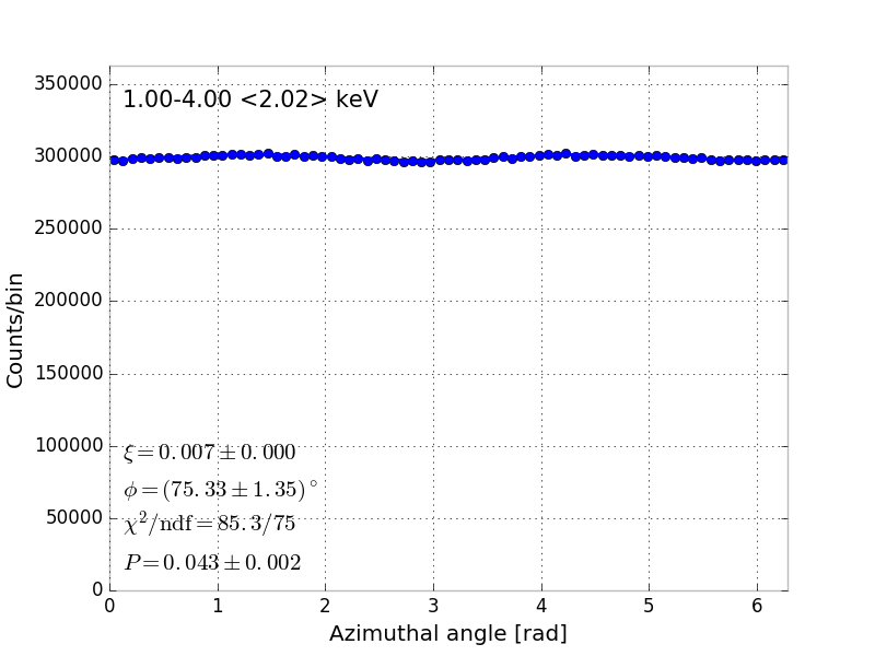
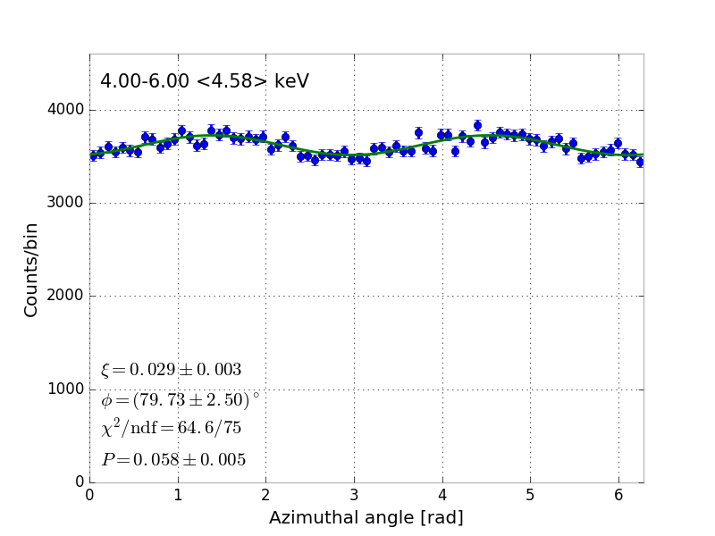
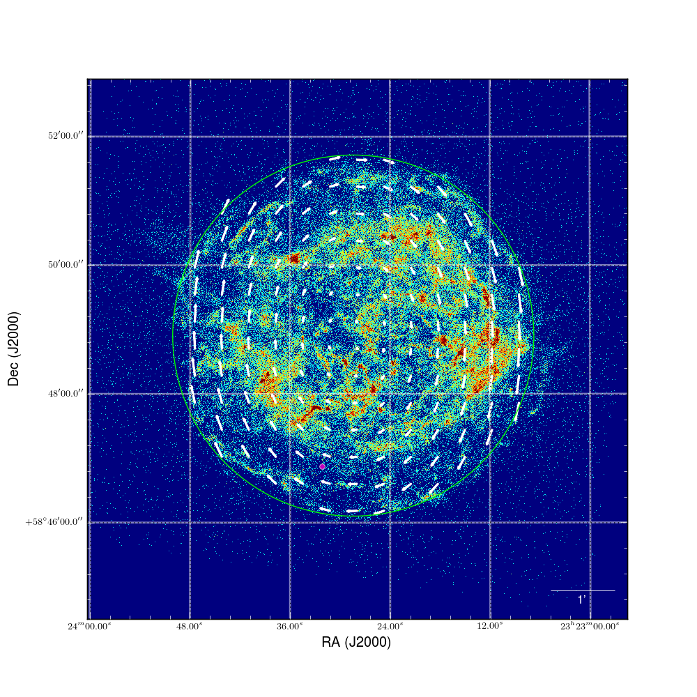
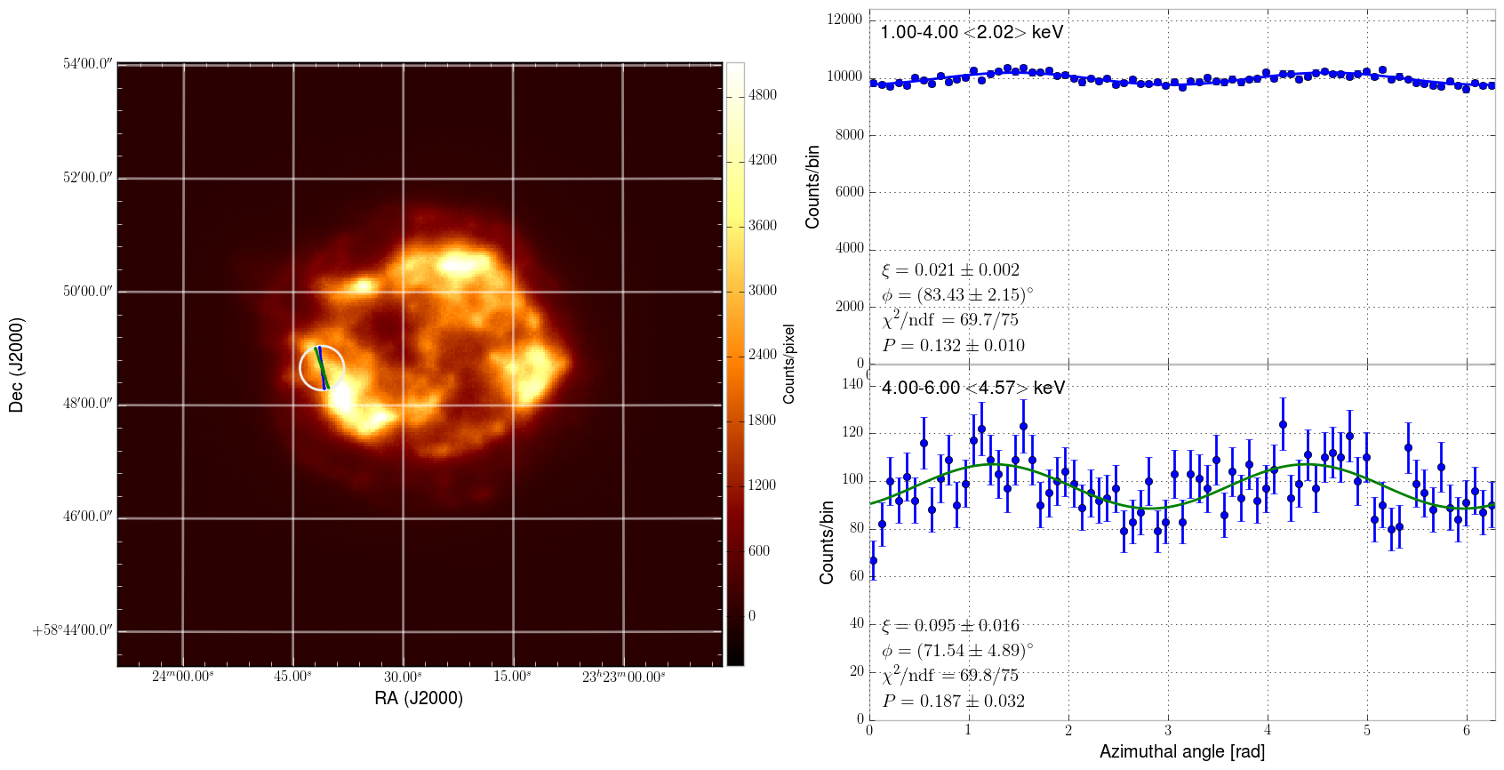
On the other hand, spatially- and energy-resolved polarimetry would in this case reveal much of the richness in the original polarization pattern. Below is an example of the azimuthal distributions in the two energy bands for the circular region of interest indicated by the white circle in the left plot. (The green and blue lines in the ROI indicate the reconstructed polarization angle.) For reference, the corresponding flux integrated in the region is about 3.5% of that of the entire source. The comparison with the previous, spatially averaged distributions is striking.

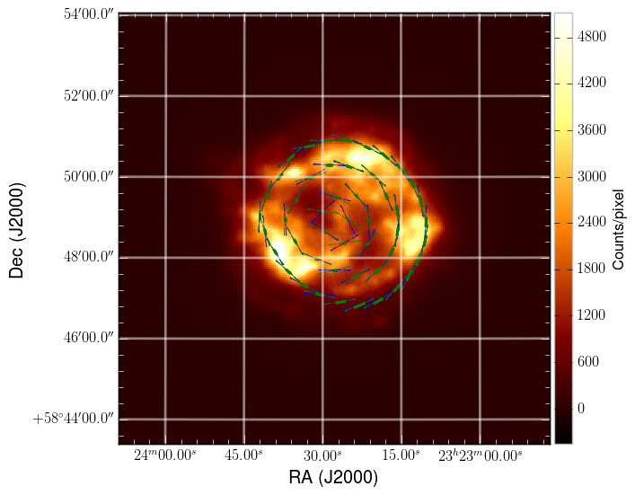
By mapping the entire field ov view with suitable regions of interest we can in fact (at least qualitatively) recover the input polarization pattern, as shown in the figre below. (Note that at the center of the image the polarization is close to zero and the arrows have little meaning.)

And below is a short animation illustrating the whole thing.

The Crab pulsar

Input model

Full source model definition in ximpol/config/crab_pulsar.py.

The input model consists of tabulated models for the phase-resolved optical polarization angle and degree and X-ray spectral parameters. The main reference we used for the compilation is Weisskopf, M. C. et al., “Chandra Phase-Resolved X-Ray Spectroscopy of the Crab Pulsar”, Astrophys. J. 743 (2011) 139–149 and essentially all the data points come from Figure 4 of this paper. The optical polarimetry data are from Słowikowska, A. et al., “Optical polarization of the Crab pulsar: precision measurements and comparison to the radio emission”, MNRAS, 397, Issue 1 (2009) 103–123.

For any specific phase value the polarization angle and degree are energy-independent (and, in the absence of X-ray data, we just assume that they are the same as the values measured in optical) and the spectral model is a simple power law (with the normalization and spectra depending on the phase). The sinusoidal parametrization of the power-law index as a function of the pulsar phase, mutuated from the reference above, is somewhat unphysical, but from our prospective is a good test of the simulation chain.

The input spatial model is simply a point source. The timing ephemeris is taken from Weisskopf, M. C. et al., “Chandra Phase-Resolved X-Ray Spectroscopy of the Crab Pulsar”, Astrophys. J. 601 (2004) 1050–1057.

Simulation output

Generation/analysis pipeline in ximpol/examples/crab_pulsar.py.

All the plots below refer to a 100 ks simulation of the Crab pulsar. (It is worth emphasizing that in this particular context we only simulate the pulsar—not the nebula. Simulating the Crab complex can surely be done within the current capabilities of the framework, but for this particular example we did not want to make the downstream analysis too complicated.)

We splitted the sample into 20 phase bins and created counts spectra (i.e., PHA1 files) and modulation cubes for each of the phase bins.

We fitted the count spectra in each phase bin with XSPEC, and the fitted parameters track reasonably well the input model. We might be seeing a slight bias in the values of the spectral index toward sistematically higher values, but overall things do look good.

We measure the average polarization degree and angle in each phase bin (we remind that the input polarization model is energy-independent) and, again, model and simulation agree well across all the phase values.

We have also simulated 100 ks of the Crab pulsar together with the nebula. Below is a short animation of the Crab complex illustrating the imaging capabilities of XIPE.

GRB 130427A

Input model

Full source model definition in ximpol/config/grb130427_swift.py.

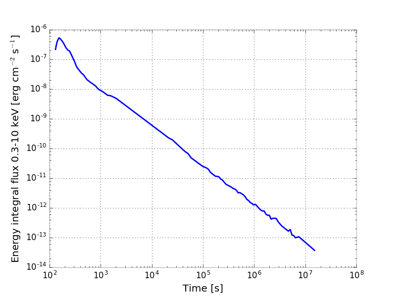
This example is meant to illustrate the simulation of a time-dependent source model. GRB 130427A (at z = 0.34) is one of the brightest GRBs ever observed in X-rays. The data points to build the light curve (shown below) are taken from the Swift XRT light-curve catalog.

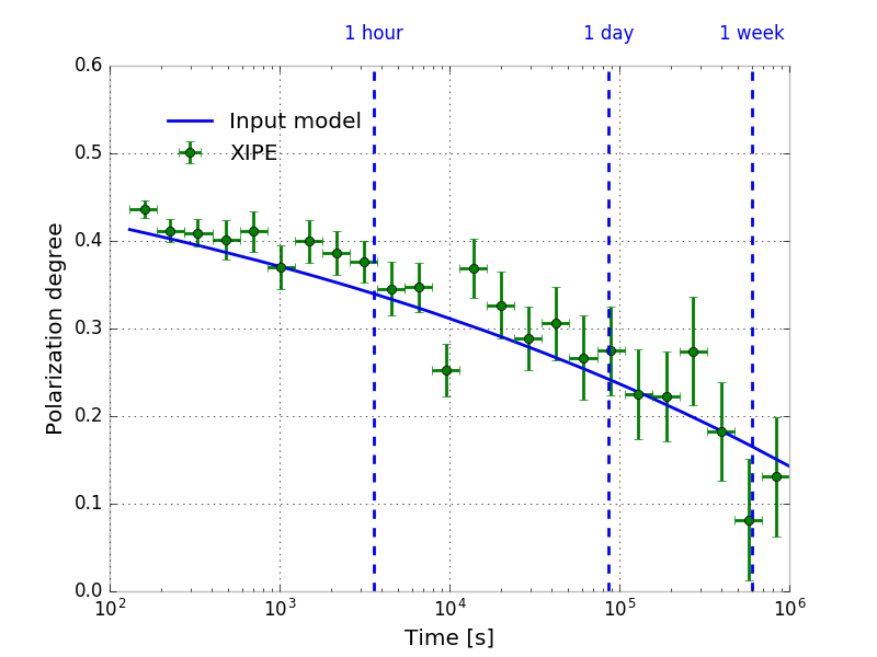
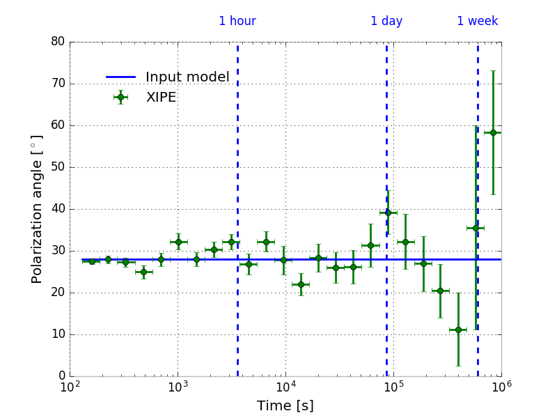
For the polarization, we made up a model where the polarization degree is decreasing with time (starting at about 40% and reaching about 10% 1 Ms after the burst) and the polarization angle is constant (see the input models in the simulation output below).

Simulation output

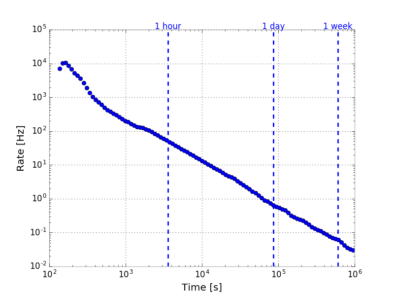
We simulated a 1 Ms observation of the GRB with XIPE. The plot below shows the count rate as a function of time.

We subselected the event file into non-overlapping time slices whose width is increasing logaritmically with time. Below are the reconstructed polarization degree and angle in each of the time bins, with the corresponding input model overlaid. Most notably, if we were able to repoint the telescope to the GRB direction within a day from the burst, we would still be sensitive to a 10–20% polarization degree in an intergration time of the order of 100 ks.