Architectural overview
The vast majority of the simulation and data preparation facilities implemented in ximpol are made available through three main executables, as illustred in the block diagram below:
xpobssim: given a source model and a set of instrument response functions, it produces a photon list correponding to a given observation time. The persistent incarnation of a photon list (that we call an event file) is binary FITS table whose format is defined inximpol.evt.event.xpselect: allows to select subsamples of photons in a given event file, based on the event energy, direction, time or phase (and, really, any of the columns in the photon list), producing a new (smaller) event file.xpbin: allows to bin the data in several different flavors, producing counts maps and spectra, light curves, phasograms and modulation cubes (i.e., histograms of the measured azimuthal distributions in multiple energy layers).
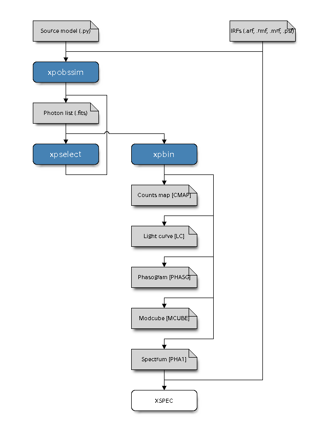
Where applicable, the data formats are consistent with the common display and analysis tools used by the community, e.g., the binned count spectra can be fed into XSPEC, along with the corresponding response functions, for doing standard spectral analysis (note that the response files used are the same for the simulation and the analysis tasks.)
All the ximpol simulation and analysis tools are fully configurable via command-line and the corresponding signatures are detailed here. In addition, ximpol provides a pipeline facility that allow to script in Python all the aforementioned functionalities (e.g., for time-resolved polarimetry this would mean: create an observation simulation for the system under study, run xpselect to split the photon list in a series of phase bins, run xpbin to create suitable modulation cubes for each of the data subselections and analyze the corresponding binned output files).
Implementation details
The basic flow of the simulation for a single model component is coded in
ximpol.srcmodel.roi.xModelComponentBase.rvs_event_list().
Notably, in order to take advantage of the efficient array manipulation
capabilities provided by numpy, the entire implementation is vectorized, i.e.
we don’t have an explicit event loop in python.
Mathematically speaking, the simulation algorith can be spelled out in the form of the following basic sequence:
Given the source spectrum
 and the effective area
 , we calculate the count spectrum as a function of
the energy and time:
, we calculate the count spectrum as a function of
the energy and time:![\mathcal{C}(E, t) = \mathcal{S}(E, t) \times A_{\rm eff}(E)
\quad [\text{s}^{-1}~\text{keV}^{-1}].](_images/math/682271e8aa92fcbbb9906658d5e615f7e89a3156.png)
We calculate the light curve of the model component (in counts space) by integrating over the energy:
![\mathcal{L}(t) = \int_{E_{\rm min}}^{E_{\rm max}} \mathcal{C}(E, t) dE
\quad [\text{Hz}].](_images/math/41c827320077046f35282f9b69014f3e8171e445.png)
We calculate the total number of expected events
 by
integrating the count rate over the observation time:
by
integrating the count rate over the observation time:
and we extract the number of observed events
 according
to a Poisson distribution with mean .
according
to a Poisson distribution with mean .We treat the count rate as a one-dimensional probability density function in the random variable
 , we extract a vector
  of values of according to this pdf—and we
sort the vector itself. (Here and in the following we shall use the hat
to indicate vectors of lenght .)
of values of according to this pdf—and we
sort the vector itself. (Here and in the following we shall use the hat
to indicate vectors of lenght .)We treat the array of count spectra
 ,
evaluated at the time array , as an array of one-dimensional
pdf objects, from which we extract a corresponding array
,
evaluated at the time array , as an array of one-dimensional
pdf objects, from which we extract a corresponding array  of
(true) energy values. (In an event-driven formulation this would
be equivalent to loop over the values
of
(true) energy values. (In an event-driven formulation this would
be equivalent to loop over the values  of the array
, calculate the corresponding count spectrum
of the array
, calculate the corresponding count spectrum
and treat that as a one-dimensional pdf from which we extract a (true) energy value
 , but the vectorized description is more germane to what
the code is actually doing internally.)
, but the vectorized description is more germane to what
the code is actually doing internally.)We treat the energy dispersion
 as an array of one-dimensional pdf objects that we use to extract
the measured energies
as an array of one-dimensional pdf objects that we use to extract
the measured energies  and the corresponding
PHA values.
and the corresponding
PHA values.We extract suitable arrays of (true)
 ,
,
 values and, similarly to what we do with the energy
dispersion, we smear them with the PSF in order to get the correponding
measured quantities.
values and, similarly to what we do with the energy
dispersion, we smear them with the PSF in order to get the correponding
measured quantities.We use the polarization degree
 and angle
  of the
model component to calculate the visibility
of the
model component to calculate the visibility  and the phase
 of the azimuthal distribution modulation, given the
modulation factor
of the azimuthal distribution modulation, given the
modulation factor  of the polarimeter
and we use these values to extract the directions of emission of the photoelectron.
(For periodic sources all of the above is done in phase, rather than in time, and the latter is recovered at the very end using the source ephemeris, but other than that there is no real difference.)
For source models involving more than one component, this is done for each component separately, and the different resulting phothon lists are then merged and ordered in time at the end of the process.