Quick start
Warning
This is now already obsolete and we should revamp it to the latest ximpol versions.
The main purpose of this simulation package is to simulate an observation of a given source model, based on suitable detector response functions.
The main Monte Carlo simulation script is ximpol/bin/xpobssim and its signature is
ximpol/bin/xpobssim.py
usage: xpobssim.py [-h] [--outfile OUTFILE] --configfile CONFIGFILE
                   [--irfname IRFNAME] [--duration DURATION] [--tstart TSTART]
                   [--seed SEED] [--vignetting {True,False}]
                   [--clobber {True,False}]
Assuming that the current working directory is the ximpol root folder, the command
ximpol/bin/xpobssim.py --configfile ximpol/config/single_point_source.py --duration 10000
should produce an event (FITS) file with a 10 ks simulation of a stationary source with a power-law spectrum (with an index of 2 and normalization of 10) with energy- and time-independent polarization degree and angle (correctly folded with all the instrument response functions: effective area, modulation factor, energy dispersion and point-spread function). The format definition for the event file is in ximpol/evt/event.py.
Now in order to bin the event file in energy (from 2 keV to 8 keV in one single bin) we run the command
ximpol/bin/xpbin.py ximpol/data/single_point_source.fits --algorithm MCUBE --emin 2. --emax 8. --ebins 1
that should produce a new FITS file (called modulation cube), containing the MDP value (at 99%) and the histogram of the azimuthal distribution of photoelectrons emission for every bin.
The binned output file can be easily visualized using the xpviewbin tool:
ximpol/bin/xpviewbin.py ximpol/data/single_point_source_mcube.fits
We are already fully equipped for a basic spectral analysis with XSPEC. The first step is to bin again the event file by running the xpbin tool with the PHA1 algorithm.
ximpol/bin/xpbin.py ximpol/data/single_point_source.fits --algorithm PHA1
Finally we can feed the binned file (along with the corresponding .arf and .rmf response functions) into XSPEC and recover the input parameters of our source.
ximpol/bin/xpxspec.py ximpol/data/single_point_source_pha1.fits
Note that xpspec.py is an example of how to use pyXspec, unfortunately not all of the XSPEC capabilties have been implemented in pyXspec (for example how to save a plot) so it is left to the user to decide whether to use XSPEC or pyXSPEC for the spectral analysis.
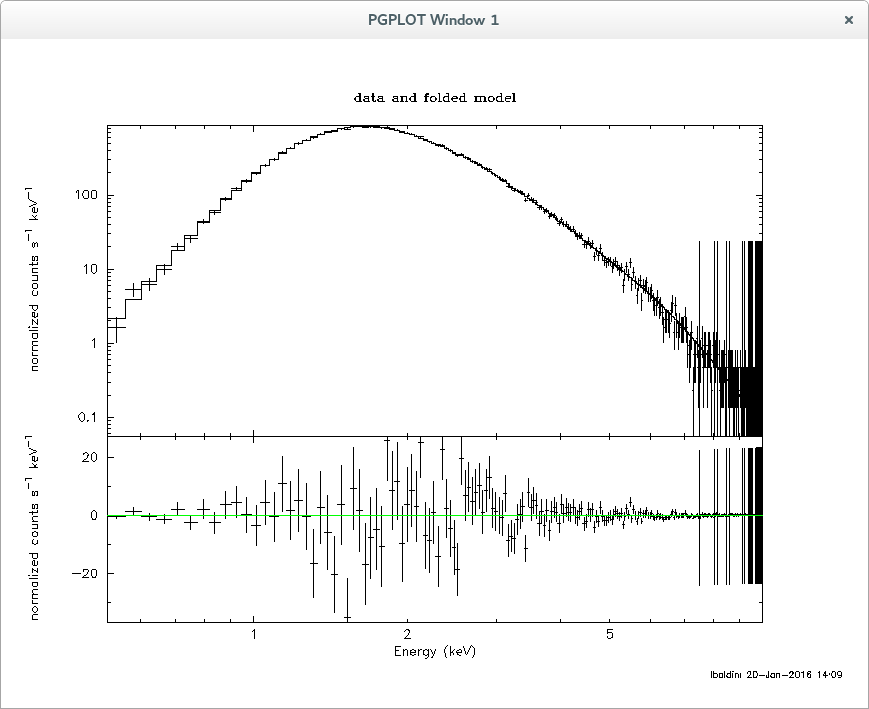
Below is the output from XSPEC on single_point_source_pha1.fits:
 Model powerlaw<1> Source No.: 1   Active/On
 Model Model Component  Parameter  Unit     Value
   par  comp
    1    1   powerlaw   PhoIndex            1.99866      +/-  7.42715E-04
    2    1   powerlaw   norm                9.99055      +/-  7.66357E-03
  ________________________________________________________________________


Fit statistic : Chi-Squared =         188.76 using 191 PHA bins.

Test statistic : Chi-Squared =         188.76 using 191 PHA bins.
 Reduced chi-squared =        0.99875 for    189 degrees of freedom
 Null hypothesis probability =   4.911785e-01