Instrument response functions (IRFs)

The instrument response functions are a crtical part of the package, and they are used (in identical form) both in the event simulation and in the analysis of the data products from the simulations.

All the response functions are stored in FITS files in the OGIP format defined in CAL/GEN/92-002 (and modifications CAL/GEN/92-002a) and are intended to be fully compatible with the spectral analysis tools provided by XSPEC (see here for more details).

We identify four different types of response functions, listed in the following table.

IRF Type	Extension	ximpol module	ximpol class
Effective area	.arf	ximpol.irf.arf	ximpol.irf.arf.xEffectiveArea
Point-spread function	.psf	ximpol.irf.psf	ximpol.irf.psf.xPointSpreadFunction
Modulation factor	.mrf	ximpol.irf.mrf	ximpol.irf.mrf.xModulationFactor
Energy dispersion	.rmf	ximpol.irf.rmf	ximpol.irf.rmf.xEnergyDispersion

(If you are familiar with basic spectral analysis in XSPEC, the .arf and .rmf files have exactly the meaning that you would expect, and can be in fact used in XSPEC).

ximpol provodes facilities for generating, reading displaying and using IRFs, as illustrated below.

Creating an IRF set: XIPE

The python module ximpol.detector.xipe.py generates a full set of instrument response functions for the baseline XIPE configuration, and it’s a sensible example of how to go about generating IRFs for arbitrary detector configurations.

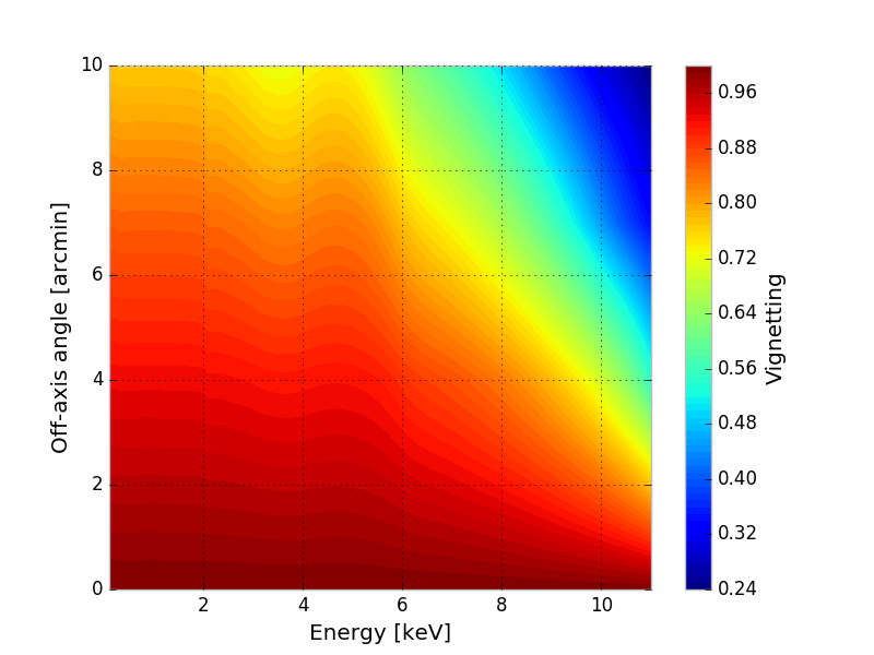
The XIPE effective area (shown in the figure below) is the product of two distinct pieces:

• The collecting area of the XIPE optics, available in aeff_optics_xipe_m4_x3.asc in ascii format. (This is the overall area for the three telescopes.)
• The quantum efficiency of the MGD in the baseline configuration (Ne/DME 80/20, 1 atm, 1 cm absorption gap), available in eff_hedme8020_1atm_1cm_cuts80p_be50um_p_x.asc. (Mind this includes the effect of the 50 um Be window and that of an energy-independent cut on the quality of the event to achieve the modulation factor predicted by the Monte Carlo.)

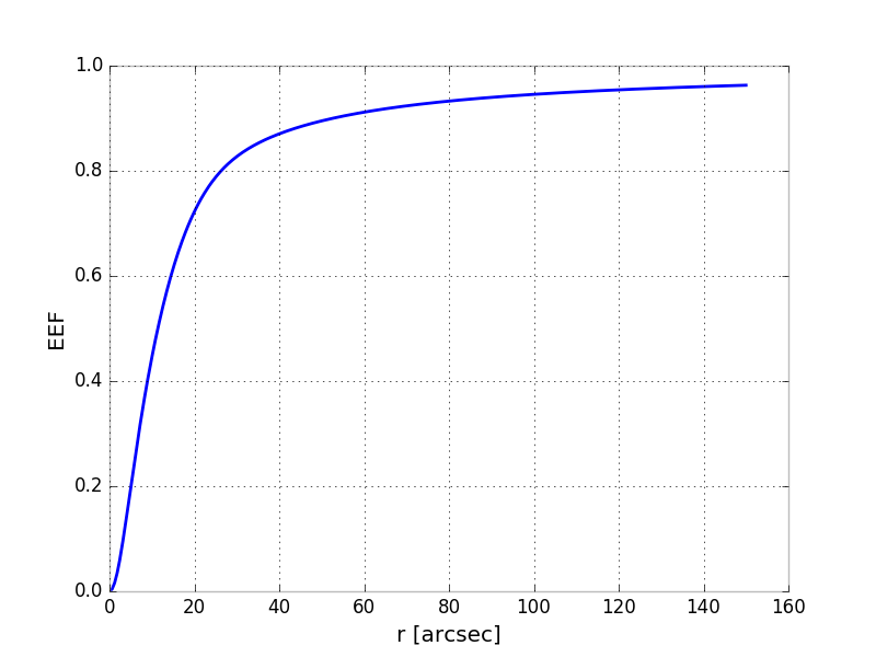
The point-spread function (PSF) is apparently difficult to estimate accurately based on the design of the optics, as it depends substantially on the defects of the surfaces (i.e., you need some metrology on the actual mirrors). For the XIPE baseline design we start by assuming a gaussian + King profile with a HEW of 15 arcsec, with the exact same parametrization and parameters values of Fabiani et al. (2014). For completeness, another paper of interest is Romano et al. (2005). Below is the actual profile of the PSF, which should be identical to Figure 6 of Fabiani at al. (2014); the parameter values were taken from Table 2 (@ 4.51 keV).

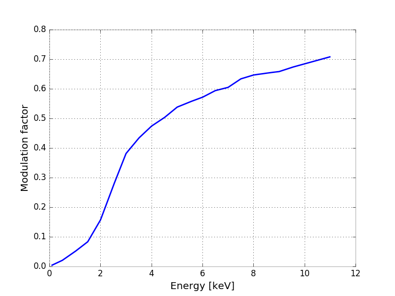
The modulation factor as a function of the energy for the relevant GPD configuration is tabulated in modfact_hedme8020_1atm_1cm_mng.asc and shown in the figure below.

The energy dispersion (i.e., the content of the .mrf FITS files) contains a two-dimensional table of the redistribution matrix in the PHA-true energy space (the MATRIX extension), and a one-dimensional table containing the correspondence between the PHA channels and the energy (the EBOUNDS extension).

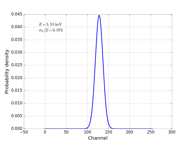
For the time being we are using a simple gaussian parametrization whose FWHM as a function of the energy is tabulated in eres_fwhm_hedme8020_1atm_1cm.asc. We’re using 256 channels between 0 and 11 keV (or 0.043 keV/channel), which seems to sample the energy dispersion adequately across the entire energy range (the typical FWHM being 1 keV or 25 channels). The MATRIX and EBOUNDS are shown in the top panel of the figure below. The bottom panel shows slices (i.e., the pdf as a function of channel) of the MATRIX at 3.73 keV and 7.36 keV.

Loading (and using) IRFs

All the instrument response functions are stored in FITS files (living in ximpol/irf/fits) and have suitable interfaces to load and use them. You can load the baseline XIPE effective area by running the following:

>>> import os
>>> from ximpol import XIMPOL_IRF
>>> from ximpol.irf.arf import xEffectiveArea
>>> file_path = os.path.join(XIMPOL_IRF, 'fits', 'xipe_baseline.arf')
>>> aeff = xEffectiveArea(file_path)

The same works for the other three IRFs. Note that XIMPOL_IRF is a convenience variable that allows you to avoid machine-dependent absolute paths and is always pointing to ximpol/irf, no matter where the package is installed. There’s many other such variables defined in ximpol.__init__.py. You can also load all four of the response functions at a time:

>>> from ximpol.irf import load_irfs
>>> aeff, psf, modf, edisp = load_irfs('xipe_baseline')

The IRFs are objects that can be evaluated at any given point—compare the outputs below with the plots at the top of the page.

>>> # Print the values of the effective area and the modulation factor and 3 keV
>>> print(aeff(3.))
>>> 164.870643616
>>> print(modf(3.))
>>> 0.380231711646
>>> # Print the value of the PSF at 20 arcsec
>>> print(psf(20.))
>>> 0.000131813525114

The energy dispersion is a somewhat more complicated object, it consists of a two-dimensional redistribution matrix and one-dimensional table containing the correspondence between the PHA channels and the energy. Below are a few examples of methods which the energy dispersion object has:

>>> # plot the 2-dimensional redistribution matrix
>>> edisp.matrix.plot()
>>> # plot a slice of the matrix at 3 keV
>>> edisp.matrix.slice(3.).plot()
>>> # plot the correspondence between the PHA channels and the energy
>>> edisp.ebounds.plot()
>>> # print the energy (in keV) corresponding to PHA channel 23
>>> print(edisp.ebounds(23))
>>> 1.009765625

Note also that the IRFs are internally represented as arrays and therefore we can also evaluate the response functions over arbitrary grids of points in one pass, e.g

>>> import numpy
>>> energy = numpy.linspace(1, 10, 10)
>>> print(energy)
>>> [  1.   2.   3.   4.   5.   6.   7.   8.   9.  10.]
>>> print(aeff(energy))
>>> [   4.9761498   305.13298991  164.87064362   68.54330826   31.6964035
>>>   16.27694702    7.43255687    3.34847045    1.49684757    0.62106234]

All of the response functions have the plot method:

>>> aeff.plot()

Most importantly, IRFs have facilities to throw random numbers according to suitable distributions to generate list of events, but this is covered in another section.

The small application bin/xpxirfview.py provides a common interface to display the content of the IRF FITS files

ximpol/bin/xpirfview.py ximpol/irf/fits/xipe_baseline.arf